This integration is designed to eliminate the need to manually move data between your spreadsheets and Cascade. It ensures your strategic data is always accurate, up-to-date, and available right where you need it, saving you valuable time on reporting and monitoring.
I. Overview: The 3-Step Connection
-
Prep Your File: Save your sheet as an .xlsx file with clean, unformatted numbers and clear, consistent dates (e.g., MM/DD/YYYY or YYYY-MM-DD).
-
Step 1 - Establish Connection: Create a secure, one-time link between your Microsoft 365 account (OneDrive/SharePoint) and your Cascade workspace.
-
Step 2 - Import Data: Select your file and metrics, specify if your data is arranged horizontally or vertically, and confirm the date column.
-
Step 3 - Configure Display: Define the Metric Name, Unit, and Time frame (e.g., Weekly, Monthly) for how the data will appear and be aggregated in Cascade.
-
Automate Tracking: The imported metric must be connected to an existing Measure in your plan to automatically update progress, and it will sync once every 24 hours.
II. Step-by-Step Configuration Guide
Get Ready to Import
Before you begin, please ensure you have:
-
A valid Cascade account and workspace.
-
A Microsoft 365 business account synced with OneDrive or SharePoint.
Preparing Your Excel File
For a perfect import, your spreadsheet needs to be in a clean, simple format. Think of it as preparing your sheet for a computer to read:
-
File Type: Your file must be saved as a standard .xlsx spreadsheet.
-
Clean Up Your Numbers: All numbers should be free of extra formatting. Do not use dollar signs ($), commas, or percentage signs (%). Formulas are fine as long as they result in a number.
-
Standardize Your Dates: Make sure all your dates are in a clear, consistent date format, such as MM/DD/YYYY or YYYY-MM-DD.
-
Maintain Your Spreadsheet Mapping: The integration relies on row and column mapping. Once you successfully import your metrics, the system maps the data to specific cells based on their position (e.g., Column C of Row 5).
-
You must not change the position of the mapped data points (dates or values) in your spreadsheet. Altering the column or row structure will cause the integration to bring in the incorrect data.
-
The Metric and Measure Connection Process
It's important to note the connection process required to automate tracking from your Excel sheets:
-
First, you must import your Excel data into the metrics in your Metrics Library.
-
Second, you then connect that metric to an existing Measure in your plan.
Once connected, your Measure will automatically update whenever new data is imported. For a full step-by-step guide on the second part of this process, please see our article: [Connect your Metrics to Measures].
Step 1: Connect Your Microsoft Excel with Cascade
First, you need to establish a connection between Cascade and Microsoft Excel. You only need to do this once. This connection can be reused for all future metric imports in your workspace.
-
Start the connection process in one of the following ways:
- Go to Metrics > Connect Metrics > Connect on Microsoft Excel
-
or, go to Metrics > Library > + Create new metric > Connect to a source.
-
Give the connection a name and click Connect.
-
Follow the instructions provided by Microsoft Office to authorize Cascade.
-
Select the specific folder or file from your OneDrive or SharePoint that you want the connection to access, or give this connection access to your entire OneDrive including all shared files.

-
Set the connection as private or shared:
-
Private (Recommended): Only you can use this connection.
-
Shared: Everyone in the workspace can use this connection.
-
-
Click Finish.
Step 2: Import Your Metrics from Excel
Now that the connection is established, you can start importing your metrics. Please note that only current and historical data can be imported into your metrics.
-
Select your Microsoft Excel connection from the list.

-
Choose the spreadsheet file and the specific sheet that contains your metrics. Click Continue.
-
Note: If you restricted access in Step 1, only those files will be listed.

-
-
Specify your spreadsheet layout: Tell Cascade if your data is arranged horizontally (across rows) or vertically (down columns). Click Next.
-
Select the metrics you want to import. Click Next.
- Note: Do not select the row or column that contains the dates.

- Select your date format and choose the exact row or column with the dates. Without dates, the import will fail. Click Next.

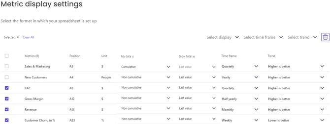
Step 3: Configure How Your Data Will Display
This is where you define how your data will be tracked and presented in Cascade.
| Metric Name | Determine the name of your metric here. Change the name of your metric if needed. |
| Unit | Specify a unit (e.g., $, %, or enter a custom unit like "Leads"). |
| My data is |
This field is for informational purposes only and does not impact your metric calculations or tracking status Select if your data is a cumulative (running total) or non-cumulative (value for a specific period). If you choose Cumulative, the "Show total as" option will automatically default to "Last value." |
| Show total as |
This field determines how your data is shown in your metrics. Sum of values: Adds up all the values for a given time period. Average of values: Calculates the average for a given time period. Last value: Shows the most recent value available in your spreadsheet. |
| Time frame | This field controls the granularity (frequency) of the data displayed on the metric graph. For example, selecting "Monthly" will display one data point per month, while "Weekly" displays one per week. Any data points beyond the selected time frame will still be stored in the metric's data table but will not appear on the visualization. |
| Trend | Define if a higher value is better (e.g., sales revenue) or a lower value is better (e.g., customer complaints). This determines the color of the metric tile (green for good, red for bad). |
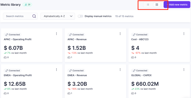
Click Connect metrics to finish the import. Your metrics will appear in the Metrics Library and will automatically sync with your Microsoft Excel every 24 hours.
Here are a couple of examples of spreadsheets that are formatted correctly for this integration:
For the image below, you would specify that your data is arranged vertical layout in Step 3.

For the image below, You would specify that your data is arranged horizontal layout in Step 3.

FAQs
What is a private and shared connection?
When a connection is set to private, only you can use this connection. When a connection is set to public", everyone in the workspace can use the same connection
How do I edit or delete a metric?
You can manage a metric through the side bar - visit Manage Existing Metrics via Sidebar
Is there a sample file I can use for the import?
Yes, you can download the sample Operating & Financial Model template from our website, input your metrics and import them into your Cascade workspace.
Can I show values for a future date?
Metrics will only display current and historical data. All data entered against a future date will be ignored.
When switching a Measure from manual to automated metric tracking, will the historical progress be retained or overwritten?
When you connect a manual Measure to a Metric, the Measure's historical progress will be overwritten by the historical data present in the spreadsheet. The spreadsheet becomes the definitive source of truth for all historical values.
I have metrics in different files, will that mean I need to do separate import every time for all these files?
Yes, but the best way is to unify them in a single spreadsheet and import in one go.
What is the data polling frequency?
The data polling frequency in case of Excel is 24 hours. It will automatically sync the data in your spreadsheet once a day, at 10 AM Sydney time.
I do not find my unit in the drop-down during import, what needs to be done?
You can add your own custom units. Just type the text, click + Add "custom unit" as a new option, and it'll get added to the list for this metric flow.
What happens if I change a value for a historical date?
The new value will simply overwrite the old data point for that specific date in the metric.
Will I see the expected progress graph and targets if I connect a Measure to a Metric?
Yes. Metrics provide the historical and current values needed to track the Measure. The expected progress is then automatically calculated based on the initial and target values you set when making the connection.
Who can use this import workflow?
Any user who has access to your Metric Library and who also has a Microsoft account with the spreadsheet saved in OneDrive or SharePoint.
Why can’t I update a Metric’s values directly within Cascade when using this integration?
We consider your Excel spreadsheet to be the single source of truth for this data. This is a one-way connection (from Excel to Cascade) designed to prevent misaligned information. Nothing you do in Cascade will change your spreadsheet values.
I get an error in Step 4 saying "Option selected is already assigned to a metric".
This happens when you've selected the row or column in which you had the dates in the previous step. Select only those metrics that you wish to import in the Mapping metrics step.
What happens when my spreadsheet is set up monthly, but I choose a quarterly timeframe during import?
If you choose a time frame larger than your source data (e.g., Quarterly over Monthly data), the values will be grouped and aggregated to fit the larger timeframe.
The data displayed will depend on the aggregation method you choose:
-
If you choose "Sum of values": The metric will add up all the monthly values within that quarter to display the quarterly total.
-
If you choose "Average of values": The metric will calculate the average of all monthly values within that quarter.
-
If you choose "Last value": The metric will display the value of the last month of that quarter (e.g., the March value for Q1).
I have formulas in my spreadsheet cells. How is this handled?
The import process fetches only the final value displayed in the cell, regardless of whether it came from a pivot table or a formula. This means it makes no difference how the value was calculated, as long as the resulting number is valid and the date is correctly formatted.
What happens if the data is set up "weekly", but I choose "monthly" in timeframe on import?
You won't see an error, but the metric will only update with a new value once per month. In the time between those updates, the same value will be displayed each week until the month changes.
I updated the progress in my spreadsheet, but the metric shows data points for a different date.
This can happen when your Time frame setting is larger than "Daily." If you choose a monthly or quarterly timeframe, your data points are grouped, and the progress will always be displayed against the last date of that period (the end of the month or the end of the quarter).
If you want to see the exact value you entered against the specific date you entered it, you must choose "Daily" in the Time frame setting.
I use the desktop application of Microsoft Excel. Will the data still sync?
This is possible, but it is important that you sync this file from your local drive to OneDrive or SharePoint. This integration will only work for files hosted on your OneDrive or a Sharepoint.